![]()
Plotting with Pandas and Matplotlib
Learning Objectives
After this lesson, you will be able to:
- Implement different types of plots on a given dataset.
Recap
In the last lesson, we learned about when to use the different types of plots. Can anyone give an example of when we would use a:
- line plot?
- bar plot?
- histogram?
- scatter plot?
Pandas and Matplotlib
As we explore different types of plots, notice:
- Different types of plots are drawn very similarly -- they even tend to share parameter names.
- In Pandas, calling
plot()on aDataFrameis different than calling it on aSeries. Although the methods are both namedplot, they may take different parameters.
Sometimes Pandas can be a little frustrating... perserverence is key!

Plotting with Pandas: How?
<data_set>.<columns>.plot()
Note: These are example plots on a ficticious dataset. We'll work with real ones in just a minute!
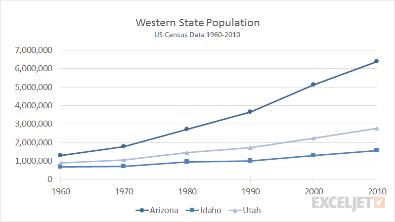
population['states'].value_counts().plot() creates:
Plotting: Visualization Types
Line charts are default.
# line chart
population['states'].value_counts().plot()
For other charts:
population['states'].plot(kind='bar')
population['states'].plot(kind='hist', bins=3);
population['states'].plot(kind='scatter', x='states', y='population')
Let's try!
Import packages
import pandas as pd
import numpy as np
import matplotlib.pyplot as plt

# set the plots to display in the Jupyter notebook
%matplotlib inline

# change plotting colors per client request
plt.style.use('ggplot')

# Increase default figure and font sizes for easier viewing.
plt.rcParams['figure.figsize'] = (8, 6)
plt.rcParams['font.size'] = 14
Load in data sets for visualization
- Football Records: International football results from 1872 to 2018
- Avocado Prices: Historical data on avocado prices and sales volume in multiple US markets
- Chocolate Bar Ratings: Expert ratings of over 1,700 chocolate bars
These have been included in ./datasets of this repo for your convenience.
!ls
foot = pd.read_csv('./international_football_results.csv')
avo = pd.read_csv('./avocado.csv')
choc = pd.read_csv('./chocolate_ratings.csv')
Let's focus on the football scores for starters.
foot.head(3)
We can extract the year by converting the date to a datetime64[ns] object, and then using the pd.Series.dt.year property to return the year (as an int). We'll learn more about this in future lessons.
foot['year'] = pd.to_datetime(foot['date']).dt.year
foot[['date', 'year']].head(3)
We can then get the number of games played every year by using pd.Series.value_counts, and using the sort_index() method to ensure our year is sorted chronologically.
foot['year'].value_counts().sort_index().head()
Using this date, we can use the pd.Series.plot() method to graph count of games against year of game:
foot['year'].value_counts().sort_index().plot();

Knowledge Check 
Why does it make sense to use a line plot for this visualization?
Another example
foot['home_team'].sort_index().value_counts().head()
Knowledge Check
Why would it NOT make sense to use a line plot for this visualization?
Count the number of games played in each country in the football dataset.
foot['country'].value_counts().head()
Let's view the same information, but in a bar chart instead. Note we are using .head() to return the top 5. Also note that value_counts() automatically sorts by the value (read the docs!)
foot['country'].value_counts().head().plot(kind='bar')

Let's change to the chocolate bar dataset.
choc.head()
How would you split the Rating values into 3 equally sized bins?
choc['Rating'].unique()
Use a histogram! The bins=n kwarg allows us to specify the number of bins ('buckets') of values.
choc.REF
# choc.select_dtypes(include='number')
plt.hist([choc['Rating'].values, choc['REF'].values], stacked=True)

choc['Rating'].plot(kind='hist', bins=3);

Sometimes it is helpful to increase this number if you think you might have an outlier or a zero-weighted set.
choc['Rating'].plot(kind='hist', bins=20)
plt.ylabel('Number of Ratings')
plt.xlabel('Chocolate Rating')
plt.title('My Title');

Knowledge check:
What does the y-axis represent on a histogram? What about the x-axis? How would you explain a histogram to a non-technical person?
Making histograms of an entire dataframe:
choc.hist(figsize=(16,8));

Why doesn't it make plots of ALL the columns in the dataframe?
Hint: what is different about the columns it plots vs. the ones it left out?
choc.head(3)
Let's take a look at the data types of all the columns:
choc.dtypes
It looks like it included REF, Review Date, and Rating. These have datatypes of int64, int64, and float64 respectively. What do these all have in common, that is different from the other data types?
Click for the answer!
They're all **numeric!** The other columns are **categorical**, specifically string values.We can filter on these types using the select_dtypes() DataFrame method (which can be very handy!)
choc.select_dtypes(include='number').head()
Challenge: create a histogram of the Review Date column, with 10 bins, and label both axes
Scatter plots are very good at showing the interaction between two numeric variables (especially when they're continuous)!
avo.head(3)
avo.plot(kind='scatter', x='Total Volume', y='AveragePrice', \
        color='dodgerblue', figsize=(10,4), s=10, alpha=0.5)

Oh snap! What did we just make?! It's a price elasticity curve!
We can also use a thing called a scatter matrix or a pairplot, which is a grid of scatter plots. This allows you to quickly view the interaction of N x M features. You are generally looking for a trend between variables (a line or curve). Using machine learning, you can fit these curves to provide predictive power.
avo.select_dtypes(include='number').iloc[:,-5:-1]
pd.plotting.scatter_matrix(
    avo.select_dtypes(include='number').iloc[:,-5:-1],
    figsize=(12,12)
);

We can also use a very handy parameter, c, which allows us to color the dots in a scatter plot. This is extremely helpful when doing classification problems, often you will set the color to the class label.
avo['type'].unique()
Let's map the type field to the color of the dot in our price elasticity curve. To use the type field, we need to convert it from a string into a number. We can use pd.Seri
Let's map the type field to the color of the dot in our price elasticity curve. To use the type field, we need to convert it from a string into a number. We can use pd.Series.apply() for this.
mapping_dict = {}
initial_class_label = 0
for type in list(avo['type'].unique()):
    mapping_dict[type] = initial_class_label
    initial_class_label += 1
mapping_dict
We can see we have two unique type labels, conventional and organic. Although that is the case for this dataset, let's create a function that will store the labels in a dictionary, incrementing the number up by 1 for each new label. This way, if we receive an additional type label in the future, our code won't break. Always think about extensible code!
Now we can use this mapping_dict dictionary to map the values using .apply():
avo['type_as_num'] = avo['type'].apply(lambda x: mapping_dict[x])
avo[['type', 'type_as_num']].head(3)
Finally, we can use this binary class label as our c parameter to gain some insight:
avo.plot(kind='scatter', x='Total Volume', y='AveragePrice', \
        c='type_as_num', colormap='winter', figsize=(8,4))
plt.xlabel('Volume')
plt.savefig('./avo_price.png');

!ls
Amazing! It looks like the organic avocados (value of 1) totally occupy the lower volume, higher price bracket. Those dang kids with their toast and unicycles driving up the price of my 'cados!
Here, we can also see a 'more' continuous c parameter, year, which makes use of the gradient a little better. There are tons of gradients you can use, check them out here.
Finally, we can save the plot to a file, using the plt.savefig() method:
Summary
In this lesson, we showed examples of how to create a variety of plots using Pandas and Matplotlib. We also showed how to use each plot to effectively display data.
Do not be concerned if you do not remember everything — this will come with practice! Although there are many plot styles, many similarities exist between how each plot is drawn. For example, they have most parameters in common, and the same Matplotlib functions are used to modify the plot area.
We looked at:
- Line plots
- Bar plots
- Histograms
- Scatter plots
Additional Resources
Always read the documentation!