Pandas is an open-source Python library of data structures and tools for exploratory data analysis (EDA). Pandas primarily facilitates acquisition, cleaning, formatting, and manipulating. Used in tandem with NumPy, Matplotlib, SciPy, and other Python libraries, Pandas is an integral part of practicing data science.

To gain some baseline familiarity with Pandas features and pre-requisites, in this lesson, you'll learn about:

• Capabilities of Pandas
• NumPy ndarray Objects
• Basic Pandas Objects
  • Index
  • Series
  • DataFrames
• Setting Up Your First Data Science Project

• Robust IO tools to reading from flat files (CSV and TXT), JSON, XML, Excel files, SQL tables, and other databases.
• Inserting and deleting columns in DataFrame and higher dimensional objects
• Handling missing data in both floating point and non-floating point data sets
• Merging & joining datasets
• Reshaping and pivoting datasets
• Conditional data sorting and filtering
• Iterating through data sets
• Aggregating and transforming data sets with split-apply-combine operations from the group by engine
• Automatic and explicit aligning and manipulating of high-dimensional data structures via hierarchical labeling and axis indexing
• Subsetting, fancy indexing, and label-based slicing large data sets
• Time-series functionality such as date range generation, date shifting, lagging, frequency conversions, moving window statistics, and moving window linear regressions.

Because Pandas is built on top of NumPy, new users should first understand one NumPy data object that often appears within Pandas objects - the ndarray.

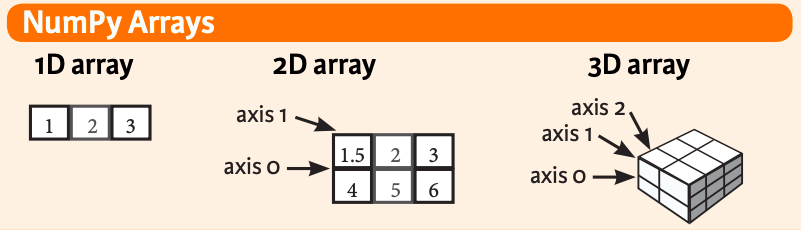
An ndarray, or N-dimensional array, is a data type from the NumPy library. Ndarrays are deceptively similar to the more general Python list type we've been working with. An ndarray type is a group of elements, which can be accessed and updated using a zero-based index. Sounds exactly like a list, right? You can create and print an ndarray exactly like a list. You can even create an ndarray from a list like this:

import numpy as np

listA = [1, 2, 3]
arrayA = np.array([1, 2, 3])
print(listA) # [1, 2, 3]
print(arrayA) # [1 2 3]

listB = ['a', 'b', 'c']
arrayB = np.array(listB)
print(listB) # ['a', 'b', 'c']
print(arrayB) # ['a' 'b' 'c']

However, there are several important differences to remember:

First, all ndarrays are homogenous.* All elements in an ndarray must be the same data type (e.g. integers, floats, strings, booleans, etc.). If you try to enter data that is not homogenous, the .array() function will force unity of data type. Side note - notice that ndarrays get printed out without commas.

import numpy as np

arrayC = np.array([1, 'b', True])
print(arrayC) # ['1', 'b', 'True']

arrayD = np.array([1, False])
print(arrayD) # [1 0]

Second, ndarrays have a parameter called ndmin, which allows you to specify the number of dimensions you want for your array when you create it. Here are the three key takeaways from the examples of this below.

• Notice how each dimension prints on its own line, so the ndarray looks more like a grid than a single list.
• arrayE1 and arrayE2 above are identical. This illustrates that the nddim parameter is optional. In other words, you can directly pass in multi-dimensional data without having to enter an argument for it.
• arrayF throws an error because it's missing one vital piece of syntax that arrayC1 has. Do you see it? The first parameter in the .array() method is the object (i.e. the values you want contained in the array). When you pass values for multiple dimensions of the array object into the .array() method, you separate them with commas. You have to make sure you group the dimensions and their values into a single group by adding () around them. If you don't, the .array() method might mistake the second dimension and its values for the second parameter of the .array() method.

import numpy as np

arrayE1 = np.array(([1, 2, 3], [4, 5, 6]))
print(arrayC1)
"""
[[1 2 3]
 [4 5 6]]
"""

arrayE2 = np.array(([1, 2, 3], [4, 5, 6]), ndmin = 2)
print(arrayC2)
"""
[[1 2 3]
 [4 5 6]]
"""

arrayF = np.array([1, 2, 3], [4, 5, 6])
print(arrayF) # Error

The third, and most important, difference between an array and a list is, ndarrays are designed to handle vectorized operations while a python list is not. In other words, if you apply a function to an ndarray object, the program will perform said function on each item in the array individually. If you apply a function to a list, the function to be performed on the list object as a whole.As a bonus, these vectorization capabilities also allow ndarrays take up less memory space and run faster.

import numpy as np

listG = [1, 2, 3]
arrayG = np.array(listA)

print(arrayG + 2) # [3 4 5]
print(listG + 2) # Error

There are a handful of other ways to create ndarrays, including random generation...

import numpy as np
import random

# Create an array of 5 random integers between 50 and 100. They will form a uniform distribution.
rand_array1 = np.random.randint(50,  100,  5)
print(rand_array1) # [54 86 91 61 90]

# Create a matrix of 2 rows and 3 columns, with all values between -1 and 1.
rand_array2 = np.random.rand(2, 3)
print(rand_array2)
"""
[[0.11298458 0.49065597 0.14219546]
 [0.27545168 0.87526704 0.93213146]]
"""

# Create a matrix of 2 rows and 3 columns, with all values between 0 and 1. They will form a normal distribution.
rand_array3 = np.random.randn(2, 3)
print(rand_array3)
"""
[[-0.24525306  1.9082735   0.55667231]
 [-1.17418436  0.12749887 -1.47157527]]
"""

...and via the .arange() method. This method takes the start point of the array, the end point, and (optionally) the step size. Remember that the final value will actually be one less than the specified end point.

range_array = np.arange(2, 8, 2)
print(range_array) # [2, 4, 6]

We know about the concept of an index from basic Python lists. Well, Pandas considers Index to be its own class of objects because you can customize an index in Pandas. As formally defined in the Pandas docs, an index object is an "immutable ndarray implementing an ordered, sliceable set" which is the default object for "storing axis labels for all pandas objects".

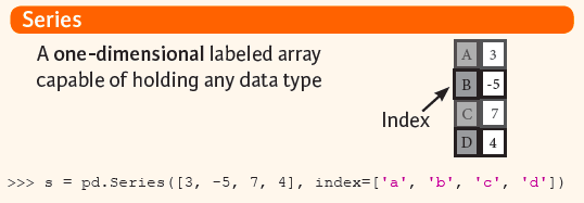
A Series is a 1-D array of data just like the Python list datatype we've been working with, but it's a bit more flexible. Some notable characteristics include:

• A Series is like a dict in that you can get and set values by index label.
• A Pandas Series acts very similarly to a NumPy ndarray:
  • Just like ndarrays, looping through a Series value-by-value is usually not necessary because of its capability to handle vectorized operations.
• The Pandas Series does have some distinct differences from an ndarray:
  • A Series can only have one dimension.
  • Operations between Series automatically align the data based on index label.

Here's the general syntax for creating a Series:

import numpy as np
import pandas as pd

s = pd.Series(data, index = index, dtype)

• The data parameter can intake a Python dict, an ndarray, or a scalar value (like 5, 7.5, True, or 'a').
• By default, the index parameter assigns an zero-based index to each element in data much like a regular Python list. Again though, you can pass custom index values to a Series to serve as axis labels for your data. Note that Pandas DOES support non-unique index values.
• dtype specifies the type of data you're passing into your Series. If you leave this blank, the program will infer the dtype from the contents of the data parameter.

Using this syntax, you can instantiate a Series from a single scalar value, a list, an ndarray, or a dict. Note: If data is an ndarray, index must be the same length as data.

import numpy as np
import pandas as pd
import random

# From a single scalar value
s_scalar = pd.Series(5., index=['a', 'b', 'c', 'd', 'e'])
"""
a    5.0
b    5.0
c    5.0
d    5.0
e    5.0
"""

# From a list
s_list = pd.Series(['red','orange','yellow','green','blue','purple'])
"""
0       red
1    orange
2    yellow
3     green
4      blue
5    purple
"""

# From an ndarray
s_ndarray = pd.Series(np.random.randn(5), index=['a', 'b', 'c', 'd', 'e'])
print(s_ndarray)
"""
a   -0.901847
b   10.503150
c    2.060891
d   -0.367695
e    1.040442
"""

# From a dict
d = {'b': 1, 'a': 0, 'c': 2} ### use wines from data set
s_dict = pd.Series(d)
"""
b    1
a    0
c    2
"""

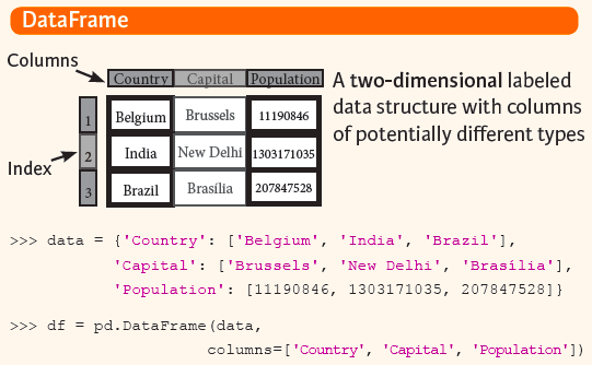
A DataFrame is a two-dimensional data matrix that stores data much like a spreadsheet does. It has labeled columns and rows with values for each column. Basically, it's virtual spreatsheet. It accepts many different data types as values, including strings, arrays (lists), dicts, Series, and even other DataFrames. The general syntax for creating a DataFrame is identical to that of a Series except it includes a second index parameter called columns parameter for adding the index values to the second dimension:

import numpy as np
import pandas as pd

df = pd.DataFrame (data, index, columns)

Creating a DataFrame is a little more complex than creating a Series because you have to consider both rows and columns. Aside from creating a dataframe indirectly by importing an existing data structure, you can create a DataFrame by:

• Specifying column names (i.e. column index values) directly within the data parameter
• Specifying column names separately in the columns parameter

import numpy as np
import pandas as pd

# Specify values for each column.
df = pd.DataFrame(
{"a" : [4 ,5, 6],
"b" : [7, 8, 9],
"c" : [10, 11, 12]},
index = [1, 2, 3])

# Specify values for each row.
df = pd.DataFrame(
[[4, 7, 10],
[5, 8, 11],
[6, 9, 12]],
index=[1, 2, 3],
columns=['a', 'b', 'c'])


# Both of these methods create a DataFrame with these values:
"""
   a   b   c
1  4   7   10
2  5   8   11
3  6   9   12
"""

Here are a few other examples:

import numpy as np
import pandas as pd

# From dict of Series or dicts
data1 = {'one': pd.Series([1., 2., 3.], index=['a', 'b', 'c']), 'two': pd.Series([1., 2., 3., 4.], index=['a', 'b', 'c', 'd'])}
df1 = pd.DataFrame(data1, index=['d', 'b', 'a'], columns=['two', 'three'])
"""
   two three
d  4.0   NaN
b  2.0   NaN
a  1.0   NaN
"""

# From dict of ndarrays / lists
data2 = {'one': [1., 2., 3., 4.],'two': [4., 3., 2., 1.]}
df2 = pd.DataFrame(data2, index=['a', 'b', 'c', 'd'])
"""
   one  two
a  1.0  4.0
b  2.0  3.0
c  3.0  2.0
d  4.0  1.0
"""

# From a list of dicts
data3 = [{'a': 1, 'b': 2}, {'a': 5, 'b': 10, 'c': 20}]
df3 = pd.DataFrame(data3, index=['first', 'second'], columns=['a', 'b', 'c'])
"""
        a   b     c
first   1   2   NaN
second  5  10  20.0
"""

Before we dive into analysis, we have to make sure we set up a stable, organized environment. For our lesson on Pandas we'll be using this dataset:

Wine Reviews | Kaggle -- 130k wine reviews with variety, location, winery, price, & description

Instead of convoluting things with a specialized Data Science IDE, we're going to start simple -- working locally, straight in the terminal. We'll walk through how to spin this up together step by step:

1) On your Desktop, create a new folder called "WineReviews". In here, we want to split up our code files from our raw data files to keep things organized.

2) Within this parent directory, create an empty "main.py" file.

3) Now, create another folder called "raw_data". Drag the wine_reviews.csv file into it.

4) Go back to the main.py file. In practice, when we go to run the main.py file in terminal, the code we'll write here will open the csv file and give the program access to its full contents.

import numpy as np 
import pandas as pd

# B) Read csv file
wine_reviews = pd.read_csv('raw_data/winemag-data-130k.csv')

First, notice that the standard is to import numpy and pandas into your python program as np and pd. Second, when you write the command to open the file, make sure you put the file name in quotes and reference the path to its location in the project directory.

5) Open up your terminal and cd into our project's parent directory.

cd ~/Desktop/WineReviews

6) Create your virtual environment

python3 -m venv .env

7) Activate the virtual environment.

source .env/bin/activate

8) Install Pandas.

pip install pandas

There are a couple salient points to mention here:

• Remember that we installed Python3 in our high-level system environment, but you don't want to do that with more specific libraries. It could cause you to run into issues if a certain version references older iterations of that library.
• For the WineReviews project, you will only have to install Pandas once. Every time you reactivate this project's virtual environment, it will have it there.
• Having NumPy installed is a pre-requisite for using Pandas. However, installing Pandas automatically installs NumPy. That's why we don't have to call pip install numpy explicitly.

9) Run the main.py file to make sure the code works!

python3 main.py

NOTE! Reading Files

We've just finished preparing our first dataset for analysis. This one was in .CSV format, but we also learned above that Pandas can handle many different file types. To open each of these in pandas we use a slightly customized version of the general method pd.read_<filetype>(<file_name>). Look here for a quick summary of commands for handling different file types in Pandas.